How buyers and sellers arrive at a price and a quantity, and what moves both when a frost, a tax, or a rent cap hits the market. The unit builds the market diagram from two straight lines, solves it, follows the coffee price through the Brazilian frost of 2021, works out who really pays a petrol tax, and ends with the trades society refuses to price, such as kidneys.
Sample unit: the complete text
On most mornings at Toyosu market in Tokyo, buyers walk along rows of frozen tuna, shine a torch on a small cut of flesh near each tail, and decide what each fish is worth to them. A few minutes later an auctioneer sells the fish one by one to the highest bidder. Nobody in the hall fixes the price in advance, yet by the end of the auction every fish has one, and the prices reflect how many fish arrived that night and how many restaurants want them. This unit explains how the same thing happens in every market, with two curves and the point where they cross, and what moves that point when a frost, a tax, or a law hits the market.
1 What a market is
A market is the set of buyers and sellers of one good, together with the way they meet and trade. The Toyosu hall is a market; so are a website on which used phones are sold, the Chicago exchange on which wheat is traded, and the petrol stations of a country, whose owners never meet but watch each other’s prices. The good can be a thing, a service, or the use of something for a while, such as a flat rented by the month.
The model of this unit describes a competitive market, which is a market with four properties. They are assumptions, and the later units relax every one of them.
There are many buyers and many sellers, each so small that no single one can move the price. Every participant is a price taker, for whom the price is a fact to react to, as the weather is for a farmer. Unit 5 studies markets in which one or a few sellers set the price.
The good is standardized, so that a buyer does not care which seller it comes from. Wheat of a given grade satisfies this; haircuts do not.
Sellers can enter and leave the market freely. Unit 4 shows what this does to prices in the long run.
Buyers and sellers know the price and the quality of what is traded. Unit 6 looks at markets in which one side knows more than the other.
Few real markets fit all four points exactly; coffee, wheat, crude oil, and shares of large companies come close, while flats, cars, and labour fit less well. The model is useful anyway, because it isolates one mechanism, the balancing of what buyers want against what sellers offer, which is at work in every market.
2 Demand and supply
2.1 Demand
The quantity demanded of a good is the amount buyers are willing and able to buy at a given price during a given interval, such as a year. It is a flow, an amount per period rather than a stock lying in a warehouse, so it always carries a time, such as million bags per year. A list of the quantities demanded at a range of prices is a demand schedule, and the same list drawn as a line is the demand curve, written \(D\) in the diagrams.
For example, the demand for coffee in the world market can be approximated, around the prices seen in 2019 and 2020, by the straight line
\[
Q_{\mathrm{d}} = 260 - 30P ,
\]
with \(P\) in US dollars per kilogram of green beans (the unroasted beans in which coffee is traded in bulk) and \(Q_{\mathrm{d}}\) in million bags of 60 kilograms per year. At a price of $3 per kilogram the world buys 170 million bags, at $4 only 140 million bags. The line is a line of best fit, chosen for the examples of this unit; the real relation is neither straight nor fixed, but near the prices that actually occurred it is a fair description.
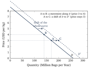
The curve slopes downwards because, as the price rises, some buyers switch to tea or drink less, and some roasters blend in cheaper beans. This is the law of demand, stated formally in the box below, and the condition attached to it matters as much as the law itself. The curve describes how the quantity demanded reacts to the price when everything else that affects buyers stays the same. When the price changes and nothing else does, the market moves along the curve. When something else changes, the whole curve moves to a new position, as Figure 1 shows. Economists keep two phrases apart for these two cases. A change in the quantity demanded is a movement along the curve, caused by a change in the good’s own price. A change in demand is a shift of the whole curve, caused by anything else.
Five things shift a demand curve.
Income. For most goods a higher income shifts demand to the right; such goods are called normal goods. For a few goods demand falls when income rises, because buyers move on to something better, and these are inferior goods, such as instant noodles or bus journeys for many households.
Prices of related goods. Two goods are substitutes when a rise in the price of one shifts the demand for the other to the right, as tea and coffee are. They are complements when they are used together, so that a rise in the price of one shifts the demand for the other to the left, as petrol and cars are.
Tastes. A health report, a fashion, or an advertising campaign moves the curve without any price changing.
Expectations. Buyers who expect a higher price next month buy more this month; buyers who expect a new model buy fewer of the old one.
The number of buyers. Market demand is the sum of individual demands, so a growing population or a newly opened export market shifts it to the right.
Figure 1. A movement along the demand curve against a shift of the curve. From A to B the price of coffee rises from $3 to $4 per kilogram and the quantity demanded falls from 170 to 140 million bags; the curve itself is unchanged. From A to C the price stays at $3 while the curve shifts to \(D'\) because, for example, incomes have risen, and 200 million bags are demanded at the old price.
2.2 Supply
The quantity supplied is the amount sellers are willing and able to sell at a given price during a given interval, and the supply curve, written \(S\), shows it for every price. For the coffee market of this unit the fitted line is
\[
Q_{\mathrm{s}} = -10 + 60P ,
\]
again in million bags per year and US dollars per kilogram. At $3 the world’s growers bring 170 million bags to market, at $4 they bring 230 million bags.
The supply curve slopes upwards for a reason that Unit 4 works out in detail. In outline, producing one more bag costs more than the last one did, because the cheapest land, the most skilled pickers, and the best machines are used first, and a higher price is needed before the more costly bag is worth producing. The height of the supply curve at any quantity is therefore the cost of producing one more item, which economists call the marginal cost; where the price covers that cost, the item is supplied.
As for demand, a change in the good’s own price moves the market along the supply curve, which is called a change in the quantity supplied, and anything else shifts the whole curve, which is called a change in supply. The shifters are the following.
Input prices. More expensive fertilizer, wages, fuel, or borrowing raise the cost of every bag and shift supply to the left.
Technology. A better harvesting machine or a disease-resistant variety lowers costs and shifts supply to the right.
Expectations. A grower who expects a higher price in six months stores beans now, which shifts today’s supply to the left.
The number of sellers. New plantations in Vietnam shifted the world supply of coffee to the right during the 1990s.
Weather and harvests. For farm goods a drought, a frost, or a disease shifts supply to the left for a season, and a good year shifts it to the right; Section 3 follows one such frost.
3 Equilibrium
3.1 The crossing point
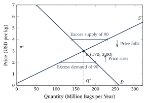
Figure 2 draws the two coffee lines in one diagram. They cross at a price of $3 per kilogram and a quantity of 170 million bags per year. At that price, and only at that price, the amount growers want to sell equals the amount buyers want to buy, and the market is in equilibrium. The equilibrium price is written \(P^{*}\) and the equilibrium quantity \(Q^{*}\).
The word equilibrium is borrowed from physics, where it means a state with no tendency to change, and that is the sense here. Consider what happens away from the crossing point. At a price of $4 per kilogram, growers would bring 230 million bags to market and buyers would take 140. The difference of 90 million bags is an excess supply, often called a surplus, a word that Section 4 uses in a second sense. Warehouses fill, and sellers who are stuck with beans offer them a little cheaper rather than keep them; as the price falls, buyers take more and growers offer less, until the gap closes. At $2 the opposite happens. Buyers want 200 million bags and growers offer 110, which leaves an excess demand of 90 million bags, a shortage. Buyers who cannot get beans bid more, the price rises, and again the gap closes. The equilibrium is stable, because any departure from it sets off a movement back towards it.
Figure 2. The market cross for the coffee lines of this unit, \(Q_{\mathrm{d}} = 260 - 30P\) and \(Q_{\mathrm{s}} = -10 + 60P\). At $4 per kilogram growers offer 230 million bags but buyers take only 140, an excess supply of 90 million bags, and unsold stocks push the price down. At $2 buyers want 200 million bags and growers offer 110, an excess demand of 90 million bags, and the price is bid up. Only at E is there no pressure on the price.
3.2 Two straight lines
When both curves are straight lines, the equilibrium can be computed rather than read off a drawing. Write the demand line as \(Q_{\mathrm{d}} = a - bP\) and the supply line as \(Q_{\mathrm{s}} = c + dP\), where \(a\), \(b\), and \(d\) are positive numbers and \(c\) may have either sign. The intercept \(a\) is the quantity buyers would take if the good were free, \(b\) says by how many bags demand falls when the price rises by one dollar, \(d\) says by how many bags supply rises for the same dollar, and \(c\) is the quantity sellers would offer at a price of zero, negative when the first bag needs a positive price before anyone grows it.
3.3 When a curve shifts
The questions economists ask of this model have the form “what happens to the price and the quantity when something changes?”, and the method for answering them is called comparative statics, which means drawing the old equilibrium, shifting the curve that the change affects, and reading off the new one. It takes three steps.
Decide which curve shifts. A change on the buyers’ side moves demand, a change on the sellers’ side moves supply, and the good’s own price moves neither.
Decide the direction. More demand or more supply at every price is a shift to the right.
Compare the new crossing point with the old one.
To see the steps at work, suppose that incomes rise. Demand shifts to the right, so at the old price of $3 buyers now want more bags than growers offer, which is an excess demand, and the price is bid up as in Section 3. As the price rises, growers move up along the unchanged supply curve and offer more, so the quantity rises together with the price.
With one curve shifting, the result is always definite, and Table 1 lists the four cases. With two curves shifting at once, one of the two answers is definite and the other depends on which shift is larger. For example, when demand rises and supply falls, as in the coffee market of 2021, the price must rise, because both shifts push it the same way, while the quantity may go either way; a reader who finds a definite answer for both has drawn one particular picture and mistaken it for the general case.
Shift
Example
Price
Quantity
Demand rises
higher incomes, a new export market
rises
rises
Demand falls
a health scare, a cheaper substitute
falls
falls
Supply rises
better technology, a good harvest
falls
rises
Supply falls
a frost, more expensive inputs, fewer sellers
rises
falls
Table 1. Comparative statics with one shifting curve. Price and quantity move together when demand shifts and in opposite directions when supply shifts, which is how an economist tells from the data which curve moved.
For straight lines the size of the move can be computed. If the supply line shifts by \(\Delta c\) (negative for a shift to the left) and nothing else changes, the equilibrium price and quantity change by
\begin{equation}
\Delta P^{*} = -\frac{\Delta c}{b + d} , \qquad \Delta Q^{*} = \frac{b\,\Delta c}{b + d} , \label{eq:shift}
\end{equation}
which follows from the key equation: with the new intercept \(c + \Delta c\) the price is \((a - c - \Delta c)/(b + d)\), and subtracting the old price \((a - c)/(b + d)\) leaves \(-\Delta c/(b + d)\); the change in the quantity then follows from \(Q^{*} = a - bP^{*}\). The same shock moves the price more when the lines are steep in the diagram, that is, when \(b\) and \(d\) are small, because a small \(b\) or \(d\) means that a dollar of price change moves the quantity only a little, so neither buyers nor sellers do much to absorb the shock. Unit 3 turns this remark into the concept of elasticity.
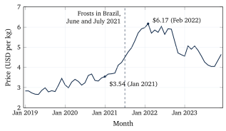
Figure 3. The monthly average price of Arabica coffee from January 2019 to December 2023 in US dollars per kilogram. The dashed line marks the frosts of June and July 2021; the price had already begun to rise with the drought and the recovery of demand after the pandemic. Source: World Bank Commodity Price Data (the Pink Sheet), series Coffee, Arabica, accessed November 2026.
4 The gains from trade
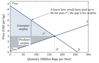
A market does more than find a price: every trade at \(P^{*}\) makes both sides better off, and the diagram measures by how much. Read the demand curve from the top down, as a list of the buyers in the order of what each would pay at most. The first bags go to whoever values coffee most, a buyer who would have paid $8 rather than go without; the buyer of the 80 millionth bag would have paid up to $6, the height of the demand curve there. Each of them pays only \(P^{*}\). The difference between what a buyer would have paid at most and what she actually pays is her gain from the trade, and the sum of these gains over all buyers is the consumer surplus. In the diagram it is the area below the demand curve and above the price line, shown in Figure 4.
The same reading works for sellers. The height of the supply curve at any quantity is the cost of producing that bag, so a grower whose bag costs $1 and who sells it for $3 gains $2. The sum over all bags sold is the producer surplus, the area above the supply curve and below the price line. The two areas together are the total surplus, the whole gain that the existence of the market creates.
Figure 4. Consumer surplus (light) and producer surplus (dark) in the coffee market of this unit. The buyer of the 80 millionth bag would have paid $6 and pays $3; her $3 is one slice of the consumer surplus. \(P_{\max}\) is the price at which demand would fall to zero and \(P_{\min}\) the price below which nothing would be supplied.
The reason economists care about these areas is a result that this unit states and Unit 6 examines. In a competitive market, the equilibrium quantity \(Q^{*}\) makes the total surplus as large as it can be, because every bag up to \(Q^{*}\) is worth more to its buyer than it costs its grower and every bag beyond it would cost more than it is worth. The proof that no other arrangement could do better goes beyond this unit. The result holds under the four assumptions of Section 1; Unit 6 shows what happens when a market harms people who are neither buyers nor sellers, as pollution does, and the crossing point is no longer the best quantity. The surplus areas are the measuring stick for what taxes and price controls do.
5 A tax on a market
Governments tax petrol, tobacco, and alcohol wholly or partly by a fixed amount per litre or packet. Suppose the tax is \(t\) per litre of petrol and the law says the petrol station must pay it. The station now needs the old price plus \(t\) to keep what it kept before, so at every quantity the supply curve sits \(t\) higher; equivalently, there is a tax wedge between the price buyers pay and the price sellers keep,
\[
P_{\mathrm{b}} - P_{\mathrm{s}} = t ,
\]
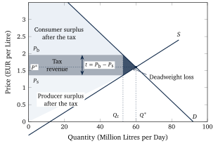
where \(P_{\mathrm{b}}\) is the price buyers pay at the pump and \(P_{\mathrm{s}}\) the amount sellers keep after sending the tax to the treasury. Figure 5 shows the new situation. The quantity traded falls to \(Q_t\), the quantity at which the demand curve is exactly \(t\) above the supply curve. Buyers pay more than before, sellers keep less than before, and the two changes add up to \(t\).
Figure 5. A tax per litre in the petrol market of this unit, drawn with a tax of 60 cents so that the areas are visible (the worked example uses 18 cents). The tax drives a wedge \(t\) between the price buyers pay, \(P_{\mathrm{b}}\), and the price sellers keep, \(P_{\mathrm{s}}\), and the quantity falls from \(Q^{*}\) to \(Q_t\). The rectangle is the tax revenue, the small dark triangle the deadweight loss, and the lighter areas are what is left of the consumer and producer surplus.
Who pays the tax? The law names the seller, but the law does not decide the matter. Economists distinguish the statutory incidence of a tax, which says who hands the money over, from its economic incidence, which says whose surplus shrinks. The diagram shows that the split depends on the slopes of the two curves. If the demand curve is steep, buyers hardly reduce their purchases when the price rises, so sellers can pass most of the tax on to them. If the supply curve is steep, sellers cannot easily cut production and have to accept a lower price themselves. It also makes no difference which side the law names: a tax collected from buyers shifts the demand curve down by \(t\) instead of the supply curve up by \(t\), and the wedge, the quantity, the two prices, and the revenue come out identical.
The tax also destroys something. Between \(Q_t\) and \(Q^{*}\) there are litres that buyers value more than they cost to produce, which is why they were traded before, and that are no longer traded because of the wedge. The surplus they would have created is lost to everyone, the treasury included, since no tax is paid on a litre that is not sold. This loss is the deadweight loss of the tax, the dark triangle in Figure 5.
6 Price ceilings and price floors
Sometimes a government, rather than taxing a market, decides that the equilibrium price is wrong and sets a legal limit on it. A price ceiling is a maximum price that may be charged, with rent control as the common case; a price floor is a minimum price that must be paid, with the minimum wage as the common case. A limit that lies on the wrong side of the equilibrium does nothing: a ceiling above \(P^{*}\) or a floor below it is not binding, because the market price obeys it anyway.
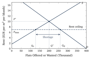
Figure 6 shows a rent ceiling. At the capped rent more households want flats, and fewer are offered, because some landlords sell their flats to people who will live in them, turn them into holiday rentals, or stop maintaining buildings that no longer pay. The gap between \(Q_{\mathrm{d}}\) and \(Q_{\mathrm{s}}\) is a shortage, and since the price may not rise to remove it, something else decides who gets the scarce flats: waiting lists, personal connections, side payments for keys or furniture, and the preferences of landlords who can now choose among many applicants. Tenants who already hold a lease at the capped rent gain. Households that need to move, newcomers, and the young lose, because the flats they would have rented at the market rent are not offered at the capped rent, and the lost trades are again a deadweight loss.
Figure 6. A rent ceiling below the equilibrium rent. At the ceiling \(P_{\max}\) tenants want \(Q_{\mathrm{d}}\) flats and landlords offer only \(Q_{\mathrm{s}}\), so the difference is a shortage that does not go away, because the price is not allowed to rise and close it. The lines are illustrative and are not fitted to a real city.
A price floor produces the mirror image. The United Kingdom’s National Living Wage, for example, is 12.71 pounds an hour for workers aged 21 and over from April 2026, and it binds in occupations whose market wage would be lower. In the simplest version of the model the workers are the sellers and the employers the buyers, with the hours of work on the horizontal axis and the wage on the vertical, and a floor above the equilibrium wage raises the hours offered by workers and lowers the hours demanded by employers, and the gap is unemployment among the affected workers: those who keep their jobs at the higher wage gain, and those who do not find work at it lose. How large the loss of jobs really is has been one of the most argued questions in economics since the study by Card and Krueger that Unit 1 described, because the answer depends on how far the labour market departs from the assumptions of Section 1; that debate goes beyond this unit.
7 Markets without prices
The model says that whenever a buyer values something more than it costs the seller, a price exists at which both gain, and that blocking the trade destroys surplus; societies nevertheless block many trades. It is illegal almost everywhere to sell a kidney, a vote, a child for adoption, a place at a public school, or a place in the queue for a transplant. The economist Alvin E. Roth has called such trades repugnant transactions: trades that some people would like to make and that others do not want them to make, even when the others are not harmed in any way the model measures. Repugnance changes with time and place: lending money at interest was repugnant in medieval Europe and is now the business of banks, and selling a human being was legal in the United States until 1865 and is unthinkable now.
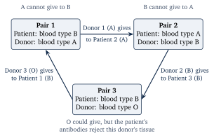
A ban on the price does not remove the scarcity. In the United States, where the National Organ Transplant Act of 1984 forbids buying or selling an organ (only the donor’s expenses may be reimbursed), more than 140,000 adult registrations were on the waiting list for a kidney at some point during 2023, a count in which a patient listed at two centres appears twice, and 4,002 patients, about eleven a day, were removed from the list that year because they had died. Many patients have a relative or friend willing to give them a kidney but cannot accept it, because the blood types do not match or because the patient’s antibodies would attack the donor’s tissue. Roth and his co-authors Tayfun Sönmez and Utku Ünver showed in 2004 how a clearing house, a central office that collects all such pairs and searches for matches among them, can match incompatible pairs with one another, so that the donor of each pair gives to the patient of another, and helped to found the first regional clearing house of this kind, the New England Program for Kidney Exchange, in 2004. Figure 7 shows the simplest cycle of three pairs. No money changes hands, each donor still gives one kidney, each patient receives one, and the trades that repugnance forbids at a price happen in kind, that is, kidney for kidney rather than for money.
Figure 7. A kidney exchange cycle of three incompatible patient-donor pairs. Within each pair the donor cannot give to his or her own patient, but each donor is compatible with the patient of the next pair, so three transplants take place at once, without any payment.
The same idea, allocation by a designed rule rather than by a price, runs through other markets society keeps money out of, such as places at public schools in New York City and Boston, which are assigned by a matching procedure that takes families’ ranked choices. Designing such rules so that people have no reason to lie about what they want is the subject of market design.
This is one of 16 units
Participants also get the quiz, the further reading, and the final exam.