Image: Böhringer Friedrich, CC BY-SA 2.5, via Wikimedia Commons
The demand curve of Unit 2 is built from a consumer's budget and preferences, and the strength of its response to price is measured with the price elasticity of demand. The unit computes elasticities from Mexico's soda tax, wheat harvests, and household food budgets, and uses them to say when a higher price raises revenue, who pays a tax, and how large the gain from a purchase is.
Preview: the beginning of the unit
On 1 January 2014 Mexico began to charge one peso on every litre of sugar-sweetened drink sold in the country, which was about 10 per cent of the shelf price at the time. During that first year, purchases of the taxed drinks fell by about 6 per cent, and by December they were 12 per cent below where they would otherwise have been. Whether such a tax cuts consumption a little or a lot, whether it raises much money for the government or stops people buying, and whether the shopper or the bottler ends up paying it, all depend on one number, the price elasticity of demand. This unit builds that number from the ground up. It starts with the question that Unit 2 left open, namely where the demand curve comes from, and it ends with a formula for the share of a tax that buyers pay.
1 The budget constraint
A consumer has a limited amount of money and must divide it between the things on offer. Economists reduce this situation to two goods, because two goods can be drawn on paper and everything learned from the drawing carries over to twenty. Call the quantities of the two goods \(x\) and \(y\), their prices \(P_x\) and \(P_y\), and the money available in the week or month under consideration \(I\), for income. If the consumer spends everything, the purchases satisfy the budget constraint\begin{equation}
P_x\,x + P_y\,y = I . \label{eq:budget}
\end{equation}
Drawn with \(x\) on the horizontal axis and \(y\) on the vertical axis, this equation is a straight line, the budget line. It meets the horizontal axis at \(I/P_x\), which is how much of good \(x\) the consumer could buy with all the money, and the vertical axis at \(I/P_y\). A pair of quantities \((x, y)\), so much of one good and so much of the other, is called a bundle. Bundles below the line leave money unspent, and bundles above it cannot be afforded.
The slope of the budget line is \(-P_x/P_y\), and this slope is the most useful thing about the drawing. It says how much of \(y\) must be given up to buy one more of \(x\). Both prices are in pounds, so the pounds cancel in the ratio, and what remains is a relative price, the price of one good measured in units of the other. The slope is therefore the opportunity cost of \(x\) in the sense of Unit 1, which means that the budget line is Unit 1’s idea of scarcity drawn for one shopper.
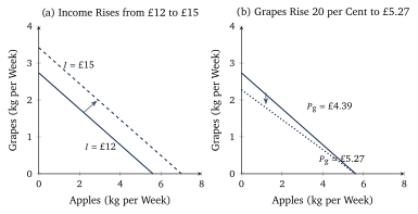
Two things move the line, a change in income and a change in one price. When income rises and prices stay the same, both intercepts grow by the same factor, so the line shifts outward parallel to itself (Figure 1a). When one price rises, only the intercept on that good’s axis moves inward, so the line pivots around the other intercept and becomes steeper or flatter (Figure 1b). A rise of all prices and of income by the same percentage leaves the line exactly where it was, because only relative prices and real income, the quantity of goods the money can buy, enter it.
Figure 1. The budget line of the worked example at the ONS average prices of January 2025. In panel (a) the weekly budget rises from 12 to 15 pounds and the line shifts outward parallel to itself. In panel (b) the price of grapes rises by 20 per cent, the apple intercept stays, and the line pivots inward around it.