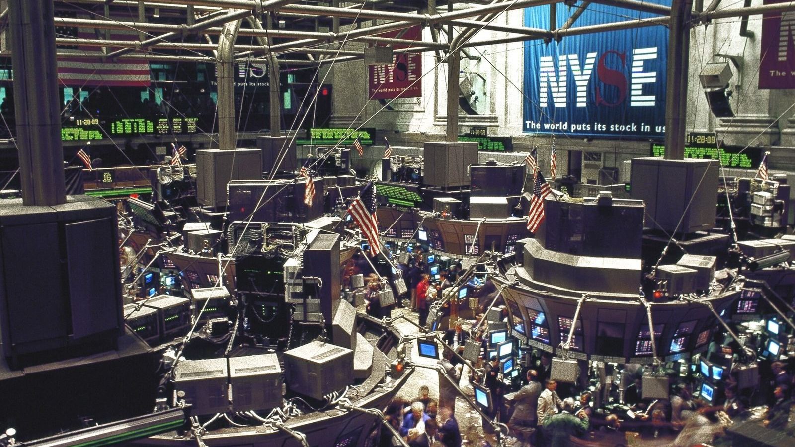
 Image: Carol M. Highsmith, Library of Congress, public domain
Why the stock market moves more than it should
In the three years from September 1929 to July 1932 the Dow Jones index fell from 381 to 41, a loss of 89 per cent. Between March 2000 and October 2002 the Nasdaq index fell by 78 per cent. Did the long-run earning power of American companies fall by four fifths in either episode? It did not; dividends fell by about half in the Depression and barely at all in 2001. The question of why prices move so much more than the payments they are a claim on is the question that founded behavioural finance, and Robert Shiller asked it in a paper published in 1981.
The efficient market and its test
In the standard model a share is worth the present value of the dividends it will pay, discounted at a rate that reflects the risk. Eugene Fama's efficient markets hypothesis of 1970 adds that the market price is the best forecast of that value given all available information, so that the price changes only when the information changes. Shiller's insight was that this claim can be tested with hindsight. We know, for every year since 1871, what dividends American companies went on to pay, so we can compute for each past date what the price would have been if investors had known the future exactly, a quantity he called the ex post rational price. The actual price is a forecast of that quantity, and a forecast should be smoother than the thing it forecasts: it moves with expectations, while the realized value moves with expectations plus every surprise. Formally, the variance of the price should be no larger than the variance of the ex post rational price. That is the variance bound.
The 1981 paper in the American Economic Review drew the two series on one chart, and the chart did the work. The ex post rational price, computed from the dividends actually paid, is a smooth line rising gently over a century. The actual price swings around it in great waves, far above it in 1929 and 1966 and far below it in 1920 and 1932. Shiller computed that the standard deviation of price changes was five to thirteen times larger than the bound allowed, depending on the assumptions. Prices were far too volatile to be forecasts of dividends.
The objections
The paper started a long argument, which is what good papers do. The variance bound assumes that the discount rate is constant, and if investors' required return moves over time, prices can move with no change in expected dividends; a generation of research on time-varying risk premia followed, and it is the main alternative explanation today. The statistics of the test were questioned, because dividends are a slowly moving series whose behaviour over a century is hard to pin down, and refined tests by Shiller with John Campbell and by others used the ratio of prices to dividends or earnings instead. The objections narrowed the claim without removing it. Fama, Lars Peter Hansen, and Shiller shared the 2013 Nobel prize in economic sciences, the Royal Swedish Academy noting that prices are unpredictable over days and partly predictable over years, which is as neat a summary of the debate as exists. Shiller's own account of what efficient markets theory could not explain, written in 2003 for the Journal of Economic Perspectives, is the research spotlight of Unit 16 of the masterclass.
CAPE
The part of the research that investors use every day is the cyclically adjusted price-earnings ratio, which Shiller and Campbell introduced in 1988 and which Shiller publishes monthly on his data page. It divides the real price of the American stock market by the average of real earnings over the previous ten years, which smooths out the swings in profits over the business cycle. The ratio has averaged about 17 since 1881. It reached 33 in September 1929, 44 in December 1999, its highest value ever, and fell to about 13 in March 2009. The point of the ratio is what it has predicted: when CAPE has been high, the real return on shares over the following ten years has been low, and when it has been low, the return has been high. The relation is loose, it says nothing about the next year, and it has been weaker since the 1990s, but a ratio in the forties has been followed by a poor decade on every occasion so far.
A worked number
The dividend discount model of Unit 16 says that the price of a share paying a dividend D next year, growing at a rate g for ever, and discounted at a rate r, is D divided by (r minus g). Take a dividend of 2 dollars, growth of 2 per cent, and a discount rate of 6 per cent: the price is 2 divided by 0.04, which is 50 dollars. Now suppose investors become a little more optimistic and raise expected growth to 2.5 per cent. The price becomes 2 divided by 0.035, which is about 57 dollars, a rise of 14 per cent from a change in a growth forecast of half a percentage point. Lower the discount rate by half a point as well, and the price is 2 divided by 0.03, or 67 dollars, a third more than where we started, with the dividend unchanged. The formula shows why prices are so sensitive to sentiment about the distant future, and why a small drift in expectations, amplified across millions of investors, can produce the waves on Shiller's chart. It does not say whether such drifts are rational revisions or moods, and that is exactly the line along which the field still divides.
What took its place
Behavioural finance did not replace the efficient market with a slogan. It added, piece by piece, the ingredients that could produce excess volatility: investors who extrapolate recent returns into the future, overconfidence that leads to overtrading, loss aversion that makes people hold losers and sell winners, herding, and the limits on the ability of better-informed investors to bet against the crowd when the crowd can stay wrong for years. Unit 16 of the masterclass, the last of the program, sets these out with the evidence for each, works through the bubbles from 1637 to 2006, and asks what policy can do. It also returns to a figure from Unit 9, the present value of a stream of payments, which is where this argument began, and asks the student to compute Shiller's two series from his own data, which is the exercise that convinced a generation of economists that something was missing from the model.